This tutorial will go over how to use histograms and boxplots in RStudio. This tutorial assumes you know the basics of R and RStudio. Please follow this series on YouTube to grasp the basics of R and RStudio.
First off, make sure you have tidyverse and cowplot installed using:
install.packages("tidyverse")
# And
install.pacakges("cowplot")
tidyverse includes the ggplot2 package which we will use the ggplot function from the package.
cowplot allows us to add multiple plots into one image.
In a new R file I have the following at the top:
library("tidyverse")
library("cowplot")

# I use an absolute path so I can run the code from any location on the computer
# and not have to worry about the relative location
coasters = read.csv("D:/Intro to Stats/Coasters_2015txt.csv")
Next we will create the necessary plots starting with the boxplot:
p1 = ggplot(coasters, aes(y = Speed)) +
  geom_boxplot()
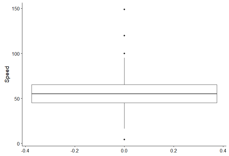
The first argument in ggplot is the data we want to give ggplot to parse. In this case the data we want is the coasters variable as that is the data loaded from our CSV. The next argument is the aes() function, short for aesthetic. We use the aes() function to tell ggplot which variables to use. We need to set the y variable for a boxplot as ggplot parses data from the y axis for a boxplot. We tell ggplot to use the Speed variable of the coasters data. To find out which variables you can use, use head(coasters) to output the first few rows of that variable. Next we add geom_boxplot() to tell ggplot to display the data as a boxplot. We put this into a variable to reference later. To view the boxplot just type in p1 into the command line, here’s how it looks currently:
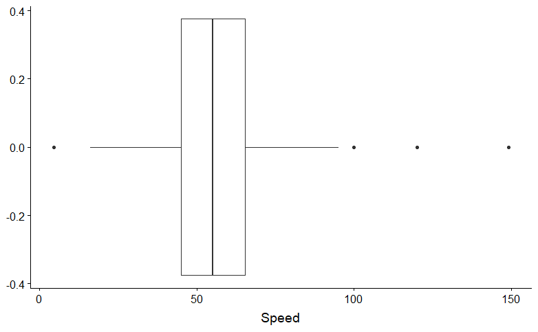
This isn’t the most ideal boxplot for our purposes as we would like it to display on top of the histogram we will make, so we want to flip it on its’ side. To do this add coord_flip() after gome_boxplot like so:
p1 = ggplot(coasters, aes(y = Speed)) +
  geom_boxplot() +
  coord_flip()
Now we get a result that we prefer:
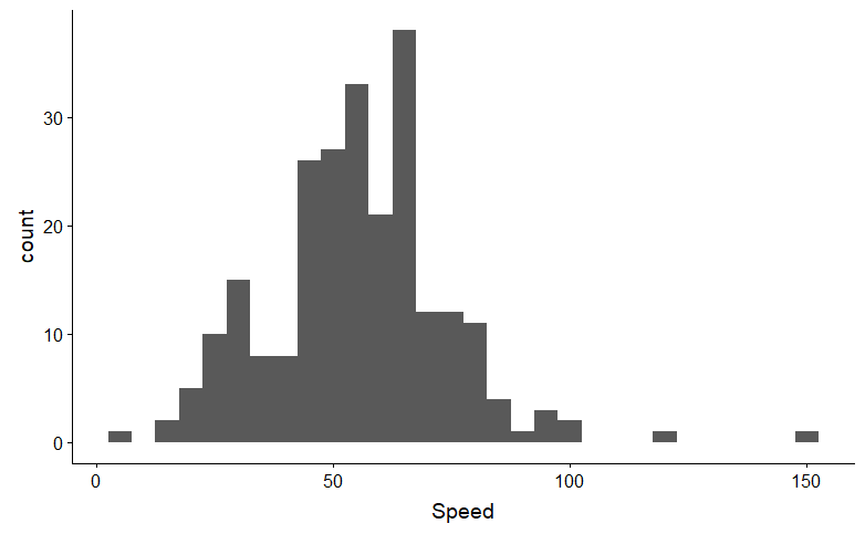
Moving on to the histogram, it will look vary similar to a the boxplot with a few tweaks. Note setting the x variable rather than the y.
p2 = ggplot(coasters, aes(x = Speed)) +
  geom_histogram(binwidth = 5)
We set x variable in aes() since geom_histogram interprets from the x variable. You can set options in geom_histogram() such as the binwidth, which we set to 5 in this example. p2 gives us this:
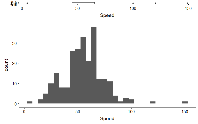
Now here comes the fun part, putting the plots together. We’ll finally use a function from cowplot to help us with this:
plot_grid(p1, p2, align = "v", ncol = 1, rel_heights = c(1, 5))
plot_grid is a function from cowplot that allows us to put multiple plots together. The first arguments of the function should be the plots that we have previously created, in this case p1 and p2 in that order, more on that later. Next we set the alignment of the plots to be vertical through align="v". Since we would like to stack the plots on top of each other, we will only need one column: ncol = 1. Finally, we set the relative heights of the plots using rel_heights = c(1, 5). rel_heights expects a vector, which we can create with the function c(). The 1 and 5 indicate the heights of the plot. The sum of the vector is 6, so imagine a part of the plot grid being 1/6 of the total height and another part 5/6 of the total height. The order of the numbers of the vector are important as well as it’s based on the plots you give it in the first part of the function. So, p1 goes with 1, and p2 goes with 5. The function should immediately output a plot like so:
While the histogram looks fine, the boxplot is squished thanks to unnecessary stuff. While you can edit rel_heights to something like rel_heights = c(1, 3) Making the boxplot bigger while making the histogram smaller. However, we can remove unnecessary elements of plots through the theme() function, which must be added to the ggplot function. First, let’s remove the X label of the boxplot using theme():
p1 = ggplot(coasters, aes(y = Speed)) +
  geom_boxplot() +
  coord_flip() +
  theme(axis.title.x = element_blank())
In the theme() function, we can set multiple parts of the plot to different elements. For this example, we set the title of the x axis to something called element_black(), which tells ggplot to remove that certain element. This addition gives us this:
This is a huge improvement than before, but it can still be improved by removing more elements:
p1 = ggplot(coasters, aes(y = Speed)) +
  geom_boxplot() +
  coord_flip() +
  theme(axis.line = element_blank(),
        axis.ticks = element_blank(),
        axis.title.y = element_blank(),
        axis.title.x = element_blank(),
        axis.text.y = element_blank())
To the theme() function, I added more arguments by removing the axis line, the axis ticks, the axis text on the y axis (the numbers), and the title on the y axis using element_blank(). Now we get the final result of:
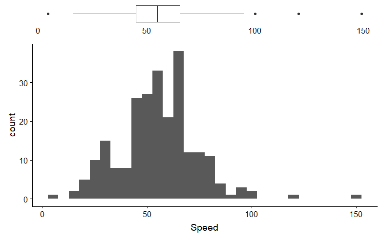
I left the numbers on the x axis of the boxplot there as a nice touch so that people can still tell where the numbers are on the boxplot without having to look at the bottom of the image.
Here is the final code:
library("tidyverse")
library("cowplot")

coasters = read.csv("D:/Intro to Stats/Coasters_2015txt.csv")

p1 = ggplot(coasters, aes(y = Speed)) +
  geom_boxplot() +
  coord_flip() +
  theme(axis.line=element_blank(),
        axis.ticks = element_blank(),
        axis.title.y=element_blank(),
        axis.title.x=element_blank(),
        axis.text.y=element_blank())

p2 = ggplot(coasters, aes(x = Speed)) +
  geom_histogram(binwidth = 5) +
  # If the lower case `count` on the histogram's y axis is bothersome,
  # you can change it using ylab()
  ylab("Count")

plot_grid(p1, p2, align = "v", ncol = 1, rel_heights = c(1, 5))